EAS439 Lab Assignment: Numerical Methods for Solving Linear Systems, ODEs, and PDEs, Singapore

Question 1

From the LU decomposition, one can derive the Jacobi and Gauss-Seidel numerical methods to iteratively solve the matrix equation.

Ax=b

These methods are important because engineering problems such as those modelled by finite difference or finite element approaches often result in this matrix equation. Typically, the matrix A is too big and sparse for the equation to be solved by analytical methods efficiently.

(a) Compose a function in MATLAB that employs the Gauss-Seidel method to solve the equation above. Your function should accept two arguments: 1) the square matrix A of any size and 2) the RHS vector b. Use a stopping criterion of εs = 0.0001% for the approximation error and a maximum iteration number of 200.

(6 marks)

(b) Calculate the solutions to the equations below using your code in part (a). Explain any modifications to each equation, if any.

(6 marks)

(c) If your function in part (a) is to employ the Jacobi method instead of Gauss-Seidel, appraise and explain the changes you have to make to the code.

(4 marks)

(d) Compute the solutions to the equations in part (b) again, this time using the Jacobi method. Which of the two methods has faster convergence? Explain a reason for the faster convergence.

(4 marks)

Question 2

The Runge-Kutta 4th-order (RK4) numerical method is a popular approach to solve ODEs of the form below due to its superior accuracy and stability over the Euler’s method.

(a) Compose a function in MATLAB that employs the RK4 method to solve the ODE above. Your function should accept the four arguments below and return a vector of times ti and a vector of solutions yi.

1. the function f(t, y),
2. the initial time t0,
3. the initial solution y0,
4. the final time tf to compute the solution until,
5. the step size h.

(4 marks)

(b) Calculate the solution to the ODE below using your code in part (a) using a step size of h = 0.1 until tf = 2. Given the exact solution yE(t), plot your numerical solution and the exact solution in one graph and appraise the relative true error of the numerical solution at tf.

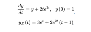
(6 marks)

(c) If the Euler’s method is used instead to solve the ODE in part (b), appraise the relative true error of the numerical solution at tf. Which numerical method is more accurate?

(4 marks)

(d) Compute the solution of the ODE below using your code in part (a) using a step size of h = 0.2 until tf = 6 and show the solution plot. Given that the exact solution is not known, explain how you would appraise the accuracy of the numerical solution at tf in this case.

(6 marks)

Question 3

The finite difference method is widely applied to solve PDEs numerically, such as the Poisson’s equation for steady-state 2D heat conduction, where f(x, y) represents a heat source.

(a) By discretizing the partial derivatives using central differences, formulate the Gauss-Seidel iterative formula to compute the temperature at node (i, j).

(6 marks)

(b) Design and program a script in MATLAB that employs the formula in part (a) to compute the solution of the Poisson’s equation. The computational parameters and boundary conditions are given below. Terminate the computation when the largest temperature difference between successive iterations is less than 1xe-6. Plot a 2D heatmap of the temperature field to show the results.

Length in x = 2 m. Length in y = 4 m. Nx = 50. Ny = 100.

Temperature at all boundaries = 25 °C. Heat source f(x, y) = 37xy.

Max iterations = 20,000.

(8 marks)

(c) Analyze the temperature field in part (b) and explain if the solution is logical.

(6 marks)

(d) Appraise the accuracy of the solution in part (b) by performing a grid convergence analysis. That is, double the mesh and compute the solution again. Compare the temperature field and the highest temperature with those in part (b) and analyse.

(4 marks)

(e) The boundary conditions are changed such that the right and top boundaries are thermally insulated. Show and explain the changes you have to make to the script in part (b). Compute the solution and show the temperature field.

(6 marks)

Question 4

The 2D unsteady heat diffusion equation with heat generation f(x, y, t) is given by, where T(x, y, t) is the temperature function of position and time.

(a) By applying Fourier’s law of heat conduction in the x and y directions given by,

formulate the above diffusion equation into the convective form below and define functions E and F clearly.

(6 marks)

(b) Formulate the finite-volume numerical scheme that is explicit in time to solve the convective equation in part (b). Define the fluxes at cell ij at time t illustrated below.

(8 marks)

(c) Design and program a script in MATLAB that employs the numerical scheme in part (b) to compute the solution of the heat diffusion equation from t = 0 to t = 3 s. The computational parameters and boundary/initial conditions are given below.

Length in x = 2 m. Length in y = 4 m. Nx = 50. Ny = 100.

Temperature at all boundaries = 25 °C. Heat source f(x, y, t) = 37xy.

Time step ∆t = 0.0004. Initial temperature at all points = 0 °C.

(8 marks)

(d) Plot a 2D heatmap of the temperature field at t = 3 s and the time evolution of the temperatures at (x, y) = (1, 1) and (x, y) = (1.2, 2.8). Analyse the plots in relation to the temperature field plotted for Question 3b.

(8 marks)